Briefly on Specific gamma ray constant and Exposure rate constant

The specific gamma ray constant $\Gamma$ is the quotient of $\displaystyle \LARGE \bf \frac{l^{2} \frac{\Delta X}{\Delta t}}{A}$

Where,
$\displaystyle \LARGE \bf l$ is the distance from point source
$\displaystyle \LARGE \bf \frac{\Delta X}{\Delta t}$ is the exposure rate
A is the activity of the nuclide

unit : R cm² h^-1 Ci^-1

The exposure rate constant $\displaystyle \LARGE \bf \Gamma_{\delta }$ has been introduced later on to replace the specific gamma ray constant $\displaystyle \LARGE \bf \Gamma$ . Specific gamma ray constant is calculated for each gamma rays emitted by radionuclide and summed. Exposure rate constant has been similarly defined but it includes all photon energies greater than $\displaystyle \LARGE \bf \delta$ , thus including the characteristic X-rays and bremsstrahlung radiation arising from conversion electrons.

$\displaystyle \LARGE \bf \Gamma_{\delta} = \Gamma + \Gamma_{x}$

where $\displaystyle \LARGE \bf \Gamma_{x}$ is the specific X-ray constant of all photons above energy $\displaystyle \LARGE \bf \delta$ , which are of non-nuclear origin

unit : R cm² h^-1 Ci^-1

Exposure rate constant and Air kerma rate constant

Though the air kema and exposure are closely related, the air kema is given by energy/mass whereas the exposure is given by charge/mass i.e. the air kerma is the measure of amount of energy transferred to secondary particle by interaction with the mass of air and they won’t concern about how secondary particle travel and how they dissipate energy, on the other hand exposure is concerned about the charge produced by secondary particle in air and how they lose all their energies (excluding bremsstrahlung).

According to ICRU 85 , Air kerma rate constant $\displaystyle \LARGE \bf \Gamma_{\delta}$ is the quotient of $\displaystyle \LARGE \bf \frac{l^{2} \dot{K}}{A}$
where, $\displaystyle \LARGE \bf \dot{K}$ is the air kerma rate due to photons above energy $\displaystyle \LARGE \bf \delta$
A is the activity of the radionuclide and $\displaystyle \LARGE \bf l$ is the distance from point source.

unit : m² Gy Bq^-1 s^-1

In below conversion , the air kerma rate constant is represented as $\displaystyle \LARGE \bf \Gamma_{AK}$

Click to access exposure_to_air_kerma.pdf

reference

Glasgow GP, Dillman LT. Specific gamma-ray constant and exposure rate constant of 192Ir. Med Phys. 1979 Jan-Feb;6(1):49-52. doi: 10.1118/1.594551. PMID: 440232.
Jayaraman, Subramania, and Lawrence H. Lanzl. Clinical radiotherapy physics. Springer Science & Business Media, 2011.
ICRU report 10 : Physical Aspects of Irradiation

Dose Volume Histogram 📈

19th May 202119th May 2021 ThirumuruganLeave a comment

Introduction

Dose volume histogram was first introduced in 1979 by Goitien and Verhey. Dose Volume Histogram (DVH) are presented as structure based DVH and non- structure based DVH. Non structure based DVH are less occasionally used and predominantly structure based DVH is used, though it has gross uncertainties in the precise location of structure. DVH are the result of statistical analysis of the discrete dose sampling points with respect to volume ( dose sampling points either be a 3D grid or randomly distributed dose sampling points).

The volume of interest is either Target, Organ At Risk (OAR), or in case of brachytherapy , it is the volume defined with relation to the implant itself.

The horizontal axis is of dose expressed (independent variable) in absolute value i.e. cGy or Gy, or-else in relative value [%] and the vertical axis is volume (dependent variable) is expressed in absolute value i.e. cc or in relative vaule [%]

Types of DVH

Differential DVH (dDVH)
Cumulative DVH (cDVH)
Natural DVH (used in brachytherapy) (nDVH)

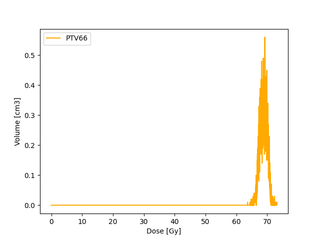
Differential DVH

It is the frequency distribution within the Volume Of Interest (VOI). The dose value are separated into specific number of bins. The bin size can be arbitrary. Then the exact number of sampling points within the each bins are calculated. Then it is multiplied with the 3D grid size if grids are used or in case of sampling points , assumed volume of each sampling is considered. Thus specific volume within each bin is obtained and plotted either as a bar graph or continuous graph.

The narrower the peak of the dDVH the more homogenous the dose distributions are within the volume of interest.

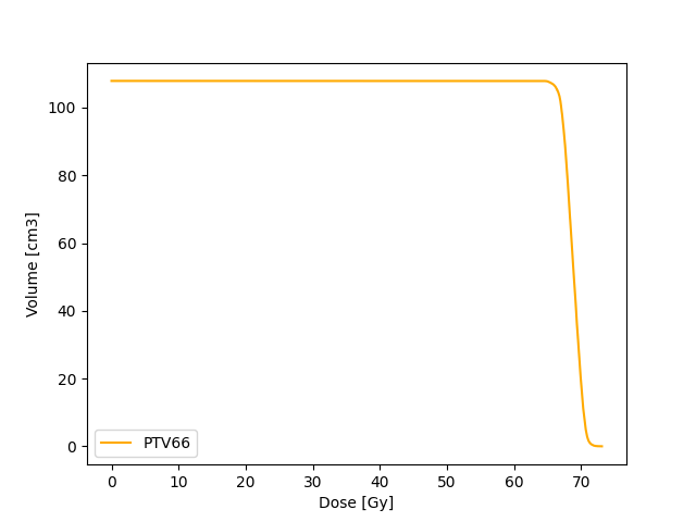
Cumulative DVH

Unlike dDVH, the cDVH represents the volume of structure receiving certain dose or higher as a function of dose. The dose and volume can either be absolute values or relative values.

The cDVH can be extracted from dDVH using $\displaystyle DVH(D) = \int_{D}^{\infty } dDVH(x)dx = 1 - \int_{0}^{D} dDVH(x)dx$

Target coverage (e.g 95 % dose is received by 100 % volume) as well as dose constraints to organ at risk (e.g. V₂₀ 30%) can be assessed with cDVH.

Natural DVH

Natural DVH is used to assess the brachytherapy plans. Below illustration of differential DVH shows the effect of inverse square law in it

The radioactive sources are placed inside the tumour or over it in case of brachytherapy. As a result the tumour is in a high dose region. The solid line in above illustration depicts the dDVH of the whole calculated structure. The vertical dotted line separated the high dose and low dose region in calculated volume. We are most interested about the information’s regarding the dose distribution such as dose homogeneity within the tumour but what we see is just a flat line in tail end of dDVH. This is due to the inverse square law effect in the dDVH (i.e. while normalizing the volume, the low dose region has more volume than high dose region, thus this suppresses the dvh in the high dose region).

To remove this effect Anderson came up with a idea on nDVH, where instead of volume, he used volume divided by dose raised to (-3/2) is used against dose.

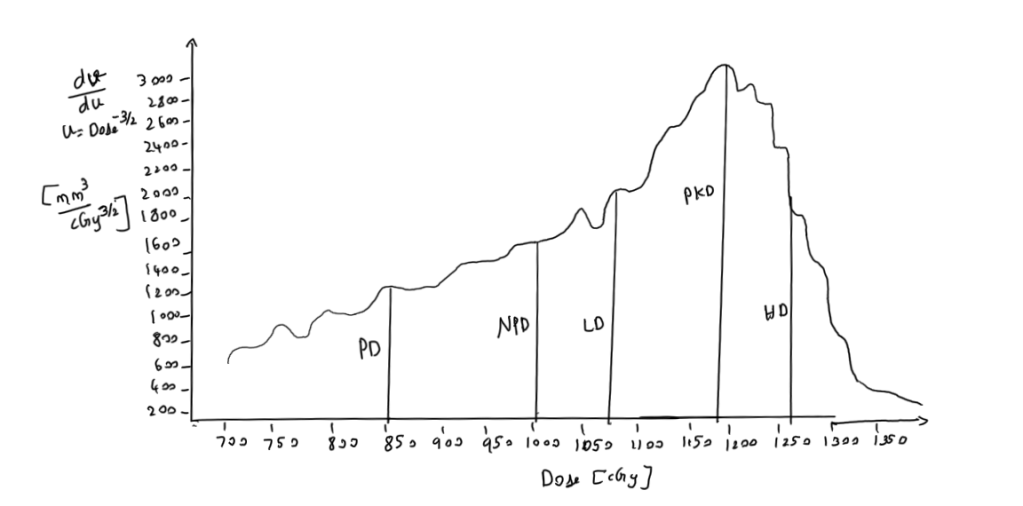
LD = Low Dose Side
HD = High Dose Side
LD and HD are dose at half maximum of the peak dose on lower side and higher dose side
PD = Prescription Dose
PkD = Peak Dose
NPD = Natural Prescription Dose
NPD is determined by steep dose decrease due to inverse square law in low dose region(i.e.) It is the dose at which low dose region stops and high dose region starts. This can be found by drawing tangents over the DVH curve
Natural Dose Ratio(NDR) = NPD/PD

Possible inferences that can be made from nDVH

Ideally PD should coincide with the LD
PD < LD produces a relatively low uniformity index
PD > LD indicates a large volume with a low dose gradient, receiving lower doses than the reference dose
Ideal NDR = 1 ; NDR > 1 overdose ; NDR < 1 under dose.

Uniformity Index is defines as

$\displaystyle UI = \frac{V(PD-HD)}{V(PD)} * \frac{u(PD)}{u(PD)-u(HD)}$

V(PD-HD) = the volume receiving a dose between PD and HD
V(PD) the volume receiving at least the prescription dose PD
u(D) =D^(-3/2)

The above expression depends on the reference dose. Manipulation of reference dose will affect the uniformity index. To overcome this influence, one more quality index was introduced by eliminating the dependence of reference dose.

$\displaystyle QI = \frac{V(LD-HD)}{V(LD)} * \frac{u(LD)}{u(LD)-u(HD)}$

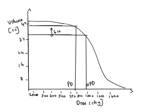
The nDVH provides assessment of uniformity and overdosage but do not provide information about target coverage. The possible way to find the target coverage is by plugging in the NPD value from nDVH into cDVH.

We have seen 3 types of DVH. DVHs have been proven to be useful tools in helping planners evaluate and compare treatment plans.

References

Bice Jr, William S. “Post Implant Evaluation.”
Moerland, Marinus A., et al. “The combined use of the natural and the cumulative dose–volume histograms in planning and evaluation of permanent prostatic seed implants.” Radiotherapy and Oncology 57.3 (2000): 279-284.
Anderson, Lowell L. “A “natural” volume–dose histogram for brachytherapy.” Medical physics 13.6 (1986): 898-903.

Linear Energy Transfer

17th Oct 202017th Oct 2020 ThirumuruganLeave a comment

The density of ionization in particle track is described by the term Linear Energy Transfer (LET). In other words, it is the measure of number of ions produced per unit path length of the track.

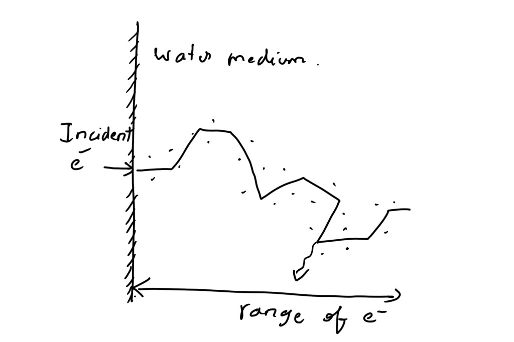
What is difference between path length and range?
The thickness of medium required for entire energy of the particle to be absorbed is called range
The entire zig-zag distance travelled is called path length

I_s = S_c/W

Where,
I_s is linear density of Ionization.
S_c is unrestricted collision stopping power
W is avg. energy expended per ionization event.

Not all energy accounted for for stopping power S_c results in ionization along the primary track. Instead some secondary electrons will have energy to travel farther away from primary track and deposit the energy. LET _Δ is defined to distinguish the ionization event occurring along the primary track from the ionization occurring due to secondary electrons farther away from primary track. The smaller the size of specific energy Δ the stricter the determination of LET _Δ with respect to ionization along primary track. The higher the Δ value the LET _Δ equals to S_c, which is represented as LET _∞(upper limit of LET).

LET is the average energy per unit distance deposited by charged particle.
Unit KeV /µm

Why LET is an average quantity?
At microscopic level the energy per unit length of track varies drastically.
(one of the complication, If the range of energy variation is too large then the average quantity itself becomes meaning less)

The definition says charged particle, but neutrons are not charged particles? How do we consider them as high- LET radiation?
The charged particles undergoes ionization by interacting with orbital electrons. In case of neutron when they pass through the tissue they do not directly produce ionization. Instead it reacts with the atomic nuclei and eject densely ionizing protons and other particles The ionization due these secondary particles results in high-LET

Different ways to calculate the average?
1] Track Average
2] Energy Average
Track Average – It is obtained by dividing the tracks into equal lengths and calculating the energy deposited in each length. It is most commonly used method
Energy Average – It is obtained by dividing the track into equal energy
intervals and averaging the lengths of the track.

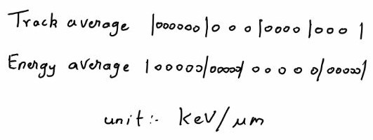
The track average and energy average is almost same for X-rays and mono energetic charged particle. In case of neutron both average shows large variation between them. The biological effects more correlated towards energy average in case of neutron.
e.g. 14 MeV neutron’s – LET track average 12 KeV /µm and energy average 100 KeV /µm

Linear Energy Transfer Values

Radiation Type	LET in KeV /µm
Cobalt – 60 γ rays	0.2
250 KV X-rays	2.0
10 MeV Protons	4.7
150 MeV Protons	0.5
14 MeV Neutrons	Track Average 12 Energy average 100
2.5 MeV α particle	166

It can be simply used to indicate the quality of radiation type(radiobiologically). It is also noted that due to above seen complication such as difference between different averaging methods and range of the average, LET may be misleading in some circumstances.

Reference
1) Hall, Eric J., and Amato J. Giaccia. Radiobiology for the Radiologist. Vol. 6. 2006.
2) Joiner, Michael C., and Albert Van der Kogel. Basic clinical radiobiology fourth edition. CRC press, 2009.
3) Jayaraman, Subramania, and Lawrence H. Lanzl. Clinical radiotherapy physics. Springer Science & Business Media, 2011.

Transport Index ☢️🚚

4th Oct 20204th Oct 2020 ThirumuruganLeave a comment

Transport index is the maximum radiation level in mSv/hr, at a distance of 1 meter from the external surface of the package, multiplied by 100

TI = Radiation level at 1m (mSv/hr) x 100

TI $\displaystyle \large \leq$ 0.05 can be considered as 0

The packages can be categorized based on the Transport Index

What is package?
The packaging with its radioactive content as presented for transport

what is packaging?
The assembly of components necessary to enclose the radioactive contents completely

Packaging + radioactive content = package

Packages are categorized based on TI into three categories
I – white
II – yellow
III – yellow
III – yellow (exclusive use)

Transport Index	Maximum dose rate on the surface	category
0	upto 5 µSv/hr	I – white
> 0 to 1	> 5 µSv/hr to 0.5 mSv/hr	II – yellow
> 1 to 10	> 0.5 mSv/hr to 2 mSv/hr	III – yellow
> 10	> 2 to mSv/hr to 10 mSv/hr	III -yellow (exclusive use)

Categories of packages

UN classification number: class 7 for radioactive materials

Reference

Rajan, KN Govinda. Radiation Safety in Radiation Oncology. CRC Press, 2017.

Radioactive decay law

26th Aug 2020 ThirumuruganLeave a comment

Radioactive decay is a stochastic process i.e. probabilistic in nature. In simple words, if we have just one unstable atom we will not know when that atom will disintegrate. But when we have a very large number of unstable atoms of same species, The decay can be estimated using probability distribution i.e. we can say with certain probability that a certain amount of radioactive nuclei will decay in a certain amount of time.

There are various modes of radioactive decay i.e. Alpha decay, beta decay and gamma decay. Though all these modes of decay are different in various aspects including the reason that causes the decay , however the number of particles that changes with time are similar for all these modes of decay.

Radioactive decay law
Here we address about single radioactive substance that’s undergoing radioactive decay to a stable daughter nucleus.

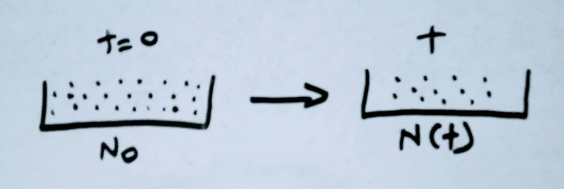
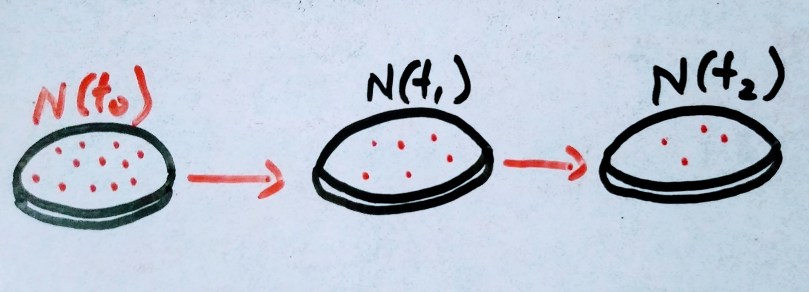
N₀ is the number of unstable atoms present at time t = 0
N is the number of atoms present at time t

The number of atoms disintegrating per unit time(dN/dt) is directly proportional to number of atoms present at a give time (N)

$\displaystyle \LARGE \bf{ \frac{\mathrm{dN} }{\mathrm{d} t} \hspace{0.3cm} \alpha \hspace{0.3cm} N}$ (eqn 1️)

The more the number of atoms present the higher the decay rate and vice versa

$\displaystyle \LARGE \bf{\frac{\mathrm{dN} }{\mathrm{d} t} \hspace{0.3cm} = \hspace{0.3cm}-\lambda N}$ (eqn 2️)

where $\displaystyle \LARGE \lambda$ is a proportionality constant (Decay constant or decay probability)
Decay probability is the probability with which any of the N radionuclides will decay.
Negative sign indicates that the rate of disintegration decreases with time i.e. the number of atoms reduces.

If we integrate equation 2 for time = 0 to time = t and find number of atoms N at time = t

$\displaystyle \huge \bf{\int_{No}^{N} \frac{\mathrm{dN} }{\mathrm{N}} = -\lambda \int_{0}^{t}dt}$ (eqn 3)

$\displaystyle \huge \bf{\log_{e}(N)-\log_{e}(No) = -\lambda t}$ (eqn 4)

$\displaystyle \huge \bf{\log_{e}(N/No) = - \lambda t}$ (eqn 5)

from basic rules of logarithm log_a (b) = c , where b = a^c
In our equation 5, b is nothing but N/No

$\displaystyle \huge \bf{\frac{N}{No} = e^{- \lambda t}}$ (eqn 6)
$\displaystyle \huge \bf{N = No \hspace{0.2cm} e^{- \lambda t}}$ (eqn 7)

Activity

Its is defined as the rate of disintegration. i.e. number of disintegration per unit time. It is given by $\displaystyle \huge \bf{ A = - \frac{\Delta N}{\Delta T} = \lambda N}$

Similar to the above equation 7 , if Ao is the initial activity at time = 0 and and A is the activity that is to be found at time = t. It is mathematically given as $\displaystyle \huge \bf{A = A_0 \hspace{0.2cm} e^{- \lambda t}}$

Half Life

The question that raises in our mind when we study about Radioactive decay is why the atoms do not decay in linear fashion. In first half life 50 % of the atoms are decayed and in next half life another remaining 50 percent of atoms are decayed , thus a complete decay happens in 2 half life?

As we discussed earlier the radioactive decay is a random process and from experimental results it is known to follow Poisson statistics. And also the exponential decay curve shows the half life idea more mathematically.
(we do postulate that atoms decay randomly, as it follows Poisson statistics but logically thinking it may or may not be if we think in reverse. Lets wait for some experiments to happen in future which may prove it)

Definition : Half life is defined as the time required for activity or atoms to decay to half of its initial value

From the equation 7 , when N = N₀ /2 and t = t_1/2 The eqn is written as

$\displaystyle \huge \bf{\frac{N_0}{2} = No \hspace{0.2cm} e^{- \lambda t_{\frac{1}{2}}}}$

from basic rules of logarithm b = a^c —-> c = log_a (b)

$\displaystyle \huge \bf{- \lambda \hspace{0.1cm} t_{\frac{1}{2}} = \ln (1) - \ln (2)}$

as ln(1) = 0 The eqn becomes $\displaystyle \huge \bf{- \lambda \hspace{0.1cm} t_{\frac{1}{2}} = - \ln (2)}$

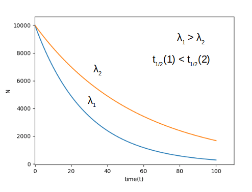
Thus half life is $\displaystyle \huge \bf{t_{\frac{1}{2}} = \frac{\ln(2)}{\lambda}}$

As the decay constant increases the half life decreases and vice versa, as seen in the above image.

Mean Life

Initially lets consider consider there are 10000 atoms of radioactive elements are there. As humans we always love to think in linear fashion. If 10 atoms decay per second initially and instead of exponential decay , the same 10 decay per second happens until the radioactive atoms vanishes. It would take 1000 seconds to completely decay. And that 1000 second is the mean life of the radioactive element.

It also turns out that mean life = half life / ln(2) . Thus for above problem we can find half life easily , where half life = mean life X ln(2). Answer turns out to be 1000 X 0.69314 = 693.14 seconds.

The Mean or average life T_a is the average lifetime for the decay of radioactive atoms.

$\displaystyle \huge \bf{T_{a} = 1 / \lambda = \frac{T_{1/2}}{ln(2)} = 1.44 \hspace{0.2cm} T_{1/2}}$

References

1 ) Khan, F. M., & Gibbons, J. P. (2014). Khan’s the physics of radiation therapy. Lippincott Williams & Wilkins.
2 ) math.ucr.edu

The time scale of effects in radiobiology 🧫

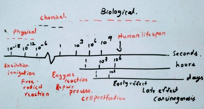
6th Jul 2020 ThirumuruganLeave a comment

The process are divided into three phases

Physical Phase
Chemical Phase
Biological Phase

Physical Phase

In physical phase the interaction between the charged particle with the atoms of the tissues occurs. It mainly interacts with orbital electrons, ejecting some of them from atoms while exciting some electrons to higher energy levels. The secondary electrons with sufficient energy can induce further ionization and excitation along the tract(cascade of ionization events). In case of indirect action the fast electrons occurs in approximately 10^-15 seconds. A high speed electrons takes about 10^-18 seconds to traverse the DNA and 10^-14 seconds to traverse the mammalian cells. for the volume of every 10 µm for 1 Gy of absorbed radiation dose almost 10⁵ ionization events occur

Incident X-ray photon
⬇️
Fast electron 10^-15 seconds

Chemical Phase

Fast electron
⬇️
Ion radical
⬇️
Free Radical
⬇️
chemical changes from breakage of bonds – 1ms(approx.)

About 80% of the cell in composed of water, when the radiation interacts with water molecules H₂O $\displaystyle \LARGE \rightarrow$ H₂O⁺ + e^– . the H₂O⁺ ion radical is formed. this ion radical further reacts with H₂O to give H₃O⁺ and OH^* where OH^* is a free radical. Free radical are highly reactive and they will undergo successive reaction to restore the electronic charge equilibrium. The free radical reactions are completed within 1 ms. The important process of chemical phase is the reactions which inactivate the free radicals e.g. reaction with sulphdryl compounds. Then the process of fixation reaction where the stable chemical changes are induced in biologically significant molecules. Here the fixation means not repair, it means that it made sure that the chemical change or damage is permanent.

Biological Phase

Chemical Changes from the breakage of bond
⬇️
Biological effect (days.months,years,
may not happen within human life span)

The biological effect occurs as the consequence of bonds broken. It begins with the enzymatic reaction that occurs on the residual chemical change. While vast majority of the cells repair, few may lead to cell death.

what is cell death? 
1) loss of specific function - differentiated cells(nerve,muscles,secretory cells) 2) loss of ability to divide - proliferating cells such as stem cells 3) loss of reproductive integrity

During the first few week and months the loss of stem cells due to the radiation is the early manifestation of normal tissue damage and the early effects are also important for tumours as they are early responding tissues.
The secondary effect of cell killing is cell proliferation, which occurs both in tumours as well as normal tissues. for normal tissue it is an important mechanism as it reduces the acute side effect
The late reactions often occur after years of radiation exposure e.g. spinal cord damage, blood vessels damage and radiation carcinogenesis

what is ion radical?

ion means electrically charged and radical means having unpaired electron in valance shell.
H₂O $\displaystyle \LARGE \rightarrow$ H₂O⁺ + e^–
H₂O⁺ is a ion radical

What is free radical?

Free radicals do not have charge but have unpaired electron in the valance shell.
H₂O⁺ + H₂O $\displaystyle \LARGE \rightarrow$ H₃O⁺ + OH^*
OH^* is the free radical

Reference
Joiner, Michael C., and Albert Van der Kogel. Basic clinical radiobiology fourth edition. CRC press, 2009.

[Most of the sentences written here are taken from basic clinical radio biology book. all credits go the authors of the book mentioned in reference ]

why do we use materials with low atomic number for shielding against neutrons 🤔

29th Jun 2020 ThirumuruganLeave a comment

Types of Neutron Interaction

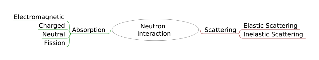
The neutron interaction is one among the major types Scattering and absorption.
In case of scattering, when the neutron interact with the nucleus the speed and direction of the neutron changes but the nucleus will be left with same number of neutron and proton as before. The energy imparted to the nucleus depends upon the angle of scattered neutron and mass of the nucleus. Eventually the nucleus will have some recoil velocity and will be in excited state that will result in the release of radiation.

The Scattering is subdivided into two types

Elastic scattering
Inelastic Scattering

Elastic Scattering

Elastic scattering is a dominant mechanism of energy deposition in case of High energy neutrons. During the interaction, as discussed earlier the fraction of neutron kinetic energy in transferred to the nucleus. The average energy loss for a neutron interacting with the nucleus of atomic weight A is $\displaystyle \large \bf{\frac {2EA}{(A+1)^2}}$ from this expression its clearly understood that we need to use a material with low atomic number.

If we use hydrogen whose atomic weight A = 1 , the average energy lost will have highest value of E/2. i.e. if the neutron is 2 MeV , because of one single elastic collision it loses energy in average about 1 MeV. and in next collision in average it loses 0.5 MeV. It almost take 27 collision in this example before in becomes thermal neutrons i.e. 0.025 eV. As the atomic number is low as well as the mass of hydrogen is comparable to neutrons. The number of interactions to reduce the energy of neutron to desired level is less

Equation to find number of collision(n) in average required to reduce initial energy of neutron E_o to the desired energy E_n is

$\displaystyle \huge \bf{\frac{log(E_n / E_0)}{log[(A^2 +1)/(A+1)^2]}}$

Inelastic Scattering

Inelastic scattering is same as that of elastic scattering expect here the nucleus undergoes internal rearrangement to go to excited state which eventually results in emission of radiation. The kinetic energy of the outgoing nucleus + neutron is less than that of incoming neutrons K.E. because some energy is lost in making the internal rearrangement of nucleus.

If the energy to make the nucleus go to excited state is very high it is highly unlikely that the inelastic collision takes place. It is the same case with hydrogen nucleus, they do not have excited states. so inelastic collisions are not possible. In general the scattering reduces(moderates) the energy of neutrons

Absorption

In case of low energy neutrons, the elastic scattering is not possible instead absorption or capture of neutrons takes place(, where the nucleus may rearrange its internal and emit one or more gamma rays or other charged particles such as protons, deuterons and alpha particles. the nucleus may also releases excess neutrons to become stable. The absorption of energy is greater than the energy of the emitted charged particles and neutrons.

Conclusion

These are the reasons why materials with low atomic numbers are used for neutron shielding which is contradictory to what we do for high energy photons, where we use high atomic number materials.

This is the reason why we use concrete barriers with combination of hydrogenous materials for construction of linac bunkers as they can shield photons, photo neutrons, and other charged particles and gamma rays that are produced while moderating neutrons. e.g. Neutron capture in hydrogen releases 2.224 MeV gamma rays.

We will look at the shielding calculations in future posts

If you want to ask any doubt or if you find any corrections to be made in this post please leave a comment below. thanks 🙂

Reference

Rinard, P. “Neutron interactions with matter.” Passive nondestructive assay of nuclear materials 375-377 (1991).

Stochastic and Non stochastic Quantities 1.1.1

27th Jun 2020 ThirumuruganLeave a comment

Let us consider a system, The system in itself is not a stochastic or non stochastic one. We define a system to be Stochastic or to be deterministic, thus it can be used to measure the physical quantities in it. In Deterministic model we assume we know everything that’s happening in the system and it can be measured using mathematical formulae and equations.

In case of Stochastic model the events happens in a random nature, Hence we find the probability distribution of the event in a particular time interval because the values vary discontinuously in space and time. The value obtained will be in some range with given probability

Where it is useful in ionizing radiation Fields 💡

The fundamental quantities in ionizing radiation are defined based on whether the process of measuring is stochastic or deterministic process

A few example of stochastic quantities defined in ICRU 85 are Energy imparted, lineal energy , specific energy, energy deposit , Where as the absorbed dose is point quantity(i.e. deterministic)

The Radioactive decay is a stochastic process, where it follows Poisson distribution which is uniquely determined by its mean value

To know more about Poisson distribution of radioactive decay refer this document by MIT click here to download and for further reading about Poisson distribution click here

Characteristics of stochastic quantity

Value/ events occurs randomly and cannot be predicted. It is determined by a probability distribution (e.g. Poisson distribution in case of radioactive decay)
It is defined for finite domains only, Its values vary discontinuously in space and time. so they do not have any gradient or rate of change
The values are found with a small uncertainty for a given probability
The expectation values X_e is the measure of its mean X̄ for n observations. as the n observation approaches ∞ the X̄ → X_e

Characteristics of Non-stochastic quantity

can be predicted using mathematical equations and formulae
It is generally a point function (e.g. absorbed dose). i.e. it has infinitesimal volumes, hence it is differentiable in space and time, rate of change can be obtained
Its value is equal to or based upon the expectation value of related stochastic quantity if one exist or they may not be related to stochastic quantity. ( e.g. Specific energy to absorbed dose where the mass is infinitesimal which we will discuss shortly)

Example

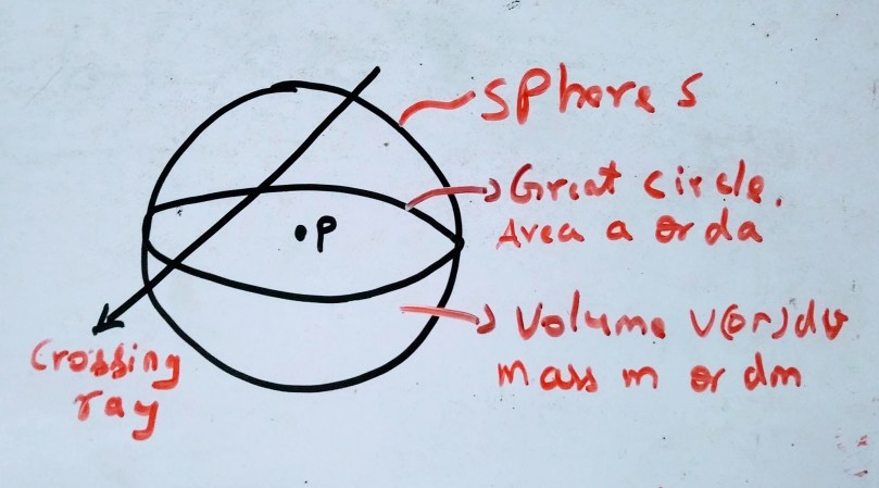
We know from the characteristics of the stochastic quantity, we need to consider a finite domain. In this case we consider a sphere because it has same cross sectional area for rays entering from any direction. Let us consider the specific energy(z), which is the quotient of energy imparted ε to the mass m, the repeated measurements will give the probability distribution of z and its mean z̄ and as the mass becomes infinitesimal dm as mentioned above in the illustration the mean z̄ approaches to absorbed dose D. (the distribution of z is actually not necessary for the measurement of D)

for example in case of biological cell it deals with micro dosimetry, where the knowledge of distribution z corresponding to a know D is important in the irradiated mass m, as the effect of radiation is more closely related to z than D. The values of z greatly differ from D for a small m

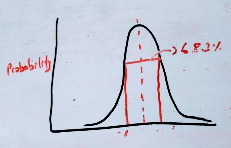
If we assume the radiation field is strictly random, as shown from above illustration the rays reaching the given point per unit area and time interval will follow Poisson distribution, for large number of events it may be approximated to Gaussian distribution

The standard deviation of single random measurement N relative to N_e is equal to σ = $\sqrt{N_e}$ $\cong$ $\sqrt{N}$ and the corresponding percentage deviation is S = $\frac{100}{\sqrt{N}}$ the single random measurement will have probability of true value falling within the uncertainty range is 68.3%

References

Wilhelm, Jochen. (2018). Re: Difference between Stochastic and Deterministic Systems (Mathematically-Physically)?. Retrieved from: https://www.researchgate.net/post/Difference_between_Stochastic_and_Deterministic_Systems_Mathematically-Physically/5a868a99f7b67eeb1a0d86ef/citation/download.
ICRU 85
Attix, Frank Herbert. Introduction to radiological physics and radiation dosimetry. John Wiley & Sons, 2008.

How is it possible for photons to transfer energy when it has no mass !

24th Jun 202024th Jun 2020 ThirumuruganLeave a comment

E = mc² is the special case of E² = ρ²c² + m²c⁴ , Its a combination of mass energy and momentum energy. The mass of photon is 0, so they get all their energy from momentum, Energy of photon reduces to E = ρc . e.g. A rope connected to an object in one end, when other end of the rope is shook violently it can move/jerk the object in other end i.e. the rope did not carry any mass but transferred energy in the form of wave motion. The same way the photons transfer energy.