Conversion of Exposure rate constant to Air kerma rate constant

Briefly on Specific gamma ray constant and Exposure rate constant

The specific gamma ray constant \Gamma is the quotient of  \displaystyle \LARGE \bf \frac{l^{2} \frac{\Delta X}{\Delta t}}{A}

Where,
 \displaystyle \LARGE \bf l is the distance from point source
 \displaystyle \LARGE \bf \frac{\Delta X}{\Delta t} is the exposure rate
A is the activity of the nuclide

unit : R cm2 h-1 Ci-1

The exposure rate constant \displaystyle \LARGE \bf \Gamma_{\delta } has been introduced later on to replace the specific gamma ray constant \displaystyle \LARGE \bf \Gamma . Specific gamma ray constant is calculated for each gamma rays emitted by radionuclide and summed. Exposure rate constant has been similarly defined but it includes all photon energies greater than \displaystyle \LARGE \bf \delta , thus including the characteristic X-rays and bremsstrahlung radiation arising from conversion electrons.

\displaystyle \LARGE \bf \Gamma_{\delta} = \Gamma + \Gamma_{x}

where \displaystyle \LARGE \bf \Gamma_{x} is the specific X-ray constant of all photons above energy \displaystyle \LARGE \bf \delta, which are of non-nuclear origin

unit : R cm2 h-1 Ci-1

Exposure rate constant and Air kerma rate constant

Though the air kema and exposure are closely related, the air kema is given by energy/mass whereas the exposure is given by charge/mass i.e. the air kerma is the measure of amount of energy transferred to secondary particle by interaction with the mass of air and they won’t concern about how secondary particle travel and how they dissipate energy, on the other hand exposure is concerned about the charge produced by secondary particle in air and how they lose all their energies (excluding bremsstrahlung).

According to ICRU 85 , Air kerma rate constant \displaystyle \LARGE \bf \Gamma_{\delta} is the quotient of \displaystyle \LARGE \bf \frac{l^{2} \dot{K}}{A}
where, \displaystyle \LARGE \bf  \dot{K} is the air kerma rate due to photons above energy \displaystyle \LARGE \bf \delta
A is the activity of the radionuclide and \displaystyle \LARGE \bf l is the distance from point source.

unit : m2 Gy Bq-1 s-1

In below conversion , the air kerma rate constant is represented as \displaystyle \LARGE \bf \Gamma_{AK}

Click to access exposure_to_air_kerma.pdf

reference

  1. Glasgow GP, Dillman LT. Specific gamma-ray constant and exposure rate constant of 192Ir. Med Phys. 1979 Jan-Feb;6(1):49-52. doi: 10.1118/1.594551. PMID: 440232.
  2. Jayaraman, Subramania, and Lawrence H. Lanzl. Clinical radiotherapy physics. Springer Science & Business Media, 2011.
  3. ICRU report 10 : Physical Aspects of Irradiation

Radioactive decay law

Radioactive decay is a stochastic process i.e. probabilistic in nature. In simple words, if we have just one unstable atom we will not know when that atom will disintegrate. But when we have a very large number of unstable atoms of same species, The decay can be estimated using probability distribution i.e. we can say with certain probability that a certain amount of radioactive nuclei will decay in a certain amount of time.

There are various modes of radioactive decay i.e. Alpha decay, beta decay and gamma decay. Though all these modes of decay are different in various aspects including the reason that causes the decay , however the number of particles that changes with time are similar for all these modes of decay.

Radioactive decay law
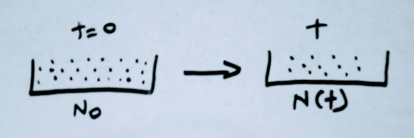
Here we address about single radioactive substance that’s undergoing radioactive decay to a stable daughter nucleus.

N0 is the number of unstable atoms present at time t = 0
N is the number of atoms present at time t

The number of atoms disintegrating per unit time(dN/dt) is directly proportional to number of atoms present at a give time (N)

\displaystyle \LARGE \bf{ \frac{\mathrm{dN} }{\mathrm{d} t} \hspace{0.3cm} \alpha \hspace{0.3cm} N} (eqn 1️)

The more the number of atoms present the higher the decay rate and vice versa

\displaystyle \LARGE \bf{\frac{\mathrm{dN} }{\mathrm{d} t} \hspace{0.3cm} = \hspace{0.3cm}-\lambda N} (eqn 2️)

where \displaystyle \LARGE \lambda is a proportionality constant (Decay constant or decay probability)
Decay probability is the probability with which any of the N radionuclides will decay.
Negative sign indicates that the rate of disintegration decreases with time i.e. the number of atoms reduces.

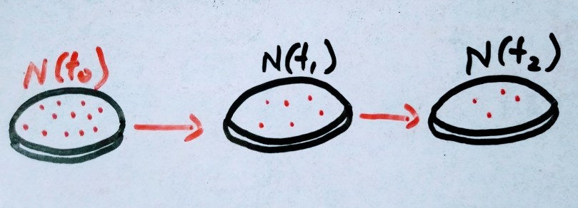
If we integrate equation 2 for time = 0 to time = t and find number of atoms N at time = t

\displaystyle \huge \bf{\int_{No}^{N} \frac{\mathrm{dN} }{\mathrm{N}} = -\lambda \int_{0}^{t}dt} (eqn 3)

\displaystyle \huge \bf{\log_{e}(N)-\log_{e}(No) = -\lambda t} (eqn 4)

\displaystyle \huge \bf{\log_{e}(N/No) = - \lambda t} (eqn 5)

from basic rules of logarithm loga (b) = c , where b = ac
In our equation 5, b is nothing but N/No

\displaystyle  \huge \bf{\frac{N}{No} = e^{- \lambda t}} (eqn 6)
\displaystyle \huge \bf{N = No \hspace{0.2cm} e^{- \lambda t}} (eqn 7)

Activity

Its is defined as the rate of disintegration. i.e. number of disintegration per unit time. It is given by \displaystyle \huge \bf{ A = - \frac{\Delta N}{\Delta T} = \lambda N}

Similar to the above equation 7 , if Ao is the initial activity at time = 0 and and A is the activity that is to be found at time = t. It is mathematically given as \displaystyle \huge \bf{A = A_0 \hspace{0.2cm} e^{- \lambda t}}

Half Life

The question that raises in our mind when we study about Radioactive decay is why the atoms do not decay in linear fashion. In first half life 50 % of the atoms are decayed and in next half life another remaining 50 percent of atoms are decayed , thus a complete decay happens in 2 half life?

As we discussed earlier the radioactive decay is a random process and from experimental results it is known to follow Poisson statistics. And also the exponential decay curve shows the half life idea more mathematically.
(we do postulate that atoms decay randomly, as it follows Poisson statistics but logically thinking it may or may not be if we think in reverse. Lets wait for some experiments to happen in future which may prove it)

Definition : Half life is defined as the time required for activity or atoms to decay to half of its initial value

From the equation 7 , when N = N0 /2 and t = t1/2 The eqn is written as

\displaystyle \huge \bf{\frac{N_0}{2}  = No \hspace{0.2cm} e^{- \lambda t_{\frac{1}{2}}}}

from basic rules of logarithm b = ac —-> c = loga (b)

\displaystyle \huge \bf{- \lambda \hspace{0.1cm} t_{\frac{1}{2}} = \ln (1) - \ln (2)}

as ln(1) = 0 The eqn becomes \displaystyle \huge \bf{- \lambda \hspace{0.1cm} t_{\frac{1}{2}} =  - \ln (2)}

Thus half life is \displaystyle \huge \bf{t_{\frac{1}{2}} = \frac{\ln(2)}{\lambda}}

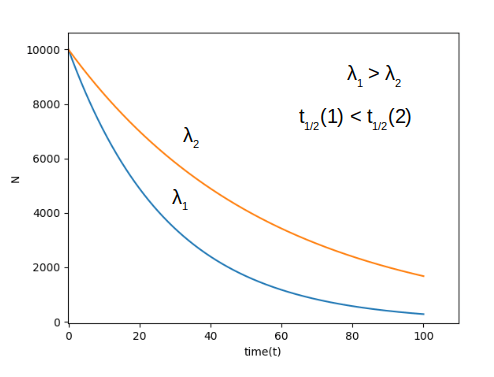
As the decay constant increases the half life decreases and vice versa, as seen in the above image.

Mean Life

Initially lets consider consider there are 10000 atoms of radioactive elements are there. As humans we always love to think in linear fashion. If 10 atoms decay per second initially and instead of exponential decay , the same 10 decay per second happens until the radioactive atoms vanishes. It would take 1000 seconds to completely decay. And that 1000 second is the mean life of the radioactive element.

It also turns out that mean life = half life / ln(2) . Thus for above problem we can find half life easily , where half life = mean life X ln(2). Answer turns out to be 1000 X 0.69314 = 693.14 seconds.

The Mean or average life Ta is the average lifetime for the decay of radioactive atoms.

\displaystyle \huge \bf{T_{a} = 1 / \lambda = \frac{T_{1/2}}{ln(2)} = 1.44 \hspace{0.2cm} T_{1/2}}

References

1 ) Khan, F. M., & Gibbons, J. P. (2014). Khan’s the physics of radiation therapy. Lippincott Williams & Wilkins.
2 ) math.ucr.edu

Stochastic and Non stochastic Quantities 1.1.1

Let us consider a system, The system in itself is not a stochastic or non stochastic one. We define a system to be Stochastic or to be deterministic, thus it can be used to measure the physical quantities in it. In Deterministic model we assume we know everything that’s happening in the system and it can be measured using mathematical formulae and equations.

In case of Stochastic model the events happens in a random nature, Hence we find the probability distribution of the event in a particular time interval because the values vary discontinuously in space and time. The value obtained will be in some range with given probability

Where it is useful in ionizing radiation Fields 💡

The fundamental quantities in ionizing radiation are defined based on whether the process of measuring is stochastic or deterministic process

A few example of stochastic quantities defined in ICRU 85 are Energy imparted, lineal energy , specific energy, energy deposit , Where as the absorbed dose is point quantity(i.e. deterministic)

The Radioactive decay is a stochastic process, where it follows Poisson distribution which is uniquely determined by its mean value

To know more about Poisson distribution of radioactive decay refer this document by MIT click here to download and for further reading about Poisson distribution click here

Characteristics of stochastic quantity

  • Value/ events occurs randomly and cannot be predicted. It is determined by a probability distribution (e.g. Poisson distribution in case of radioactive decay)
  • It is defined for finite domains only, Its values vary discontinuously in space and time. so they do not have any gradient or rate of change
  • The values are found with a small uncertainty for a given probability
  • The expectation values Xe is the measure of its mean X̄ for n observations. as the n observation approaches the X̄ → Xe

Characteristics of Non-stochastic quantity

  • can be predicted using mathematical equations and formulae
  • It is generally a point function (e.g. absorbed dose). i.e. it has infinitesimal volumes, hence it is differentiable in space and time, rate of change can be obtained
  • Its value is equal to or based upon the expectation value of related stochastic quantity if one exist or they may not be related to stochastic quantity. ( e.g. Specific energy to absorbed dose where the mass is infinitesimal which we will discuss shortly)

Example

We know from the characteristics of the stochastic quantity, we need to consider a finite domain. In this case we consider a sphere because it has same cross sectional area for rays entering from any direction. Let us consider the specific energy(z), which is the quotient of energy imparted ε to the mass m, the repeated measurements will give the probability distribution of z and its mean z̄ and as the mass becomes infinitesimal dm as mentioned above in the illustration the mean z̄ approaches to absorbed dose D. (the distribution of z is actually not necessary for the measurement of D)

for example in case of biological cell it deals with micro dosimetry, where the knowledge of distribution z corresponding to a know D is important in the irradiated mass m, as the effect of radiation is more closely related to z than D. The values of z greatly differ from D for a small m

If we assume the radiation field is strictly random, as shown from above illustration the rays reaching the given point per unit area and time interval will follow Poisson distribution, for large number of events it may be approximated to Gaussian distribution

The standard deviation of single random measurement N relative to Ne is equal to σ = \sqrt{N_e} \cong \sqrt{N} 
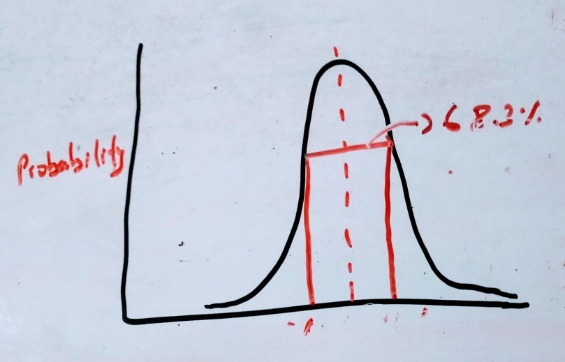
and the corresponding percentage deviation is S = \frac{100}{\sqrt{N}} the single random measurement will have probability of true value falling within the uncertainty range is 68.3%

References